Ising 2D 400 Information

Download or save the software by clicking here or on “Ising 2D 400” or the icon on the Ising front page.

Information on how to use the software is here.

The Ising model is a model of a magnet. The essential premise behind it is that the magnetism of a bulk material is made up of the combined magnetic dipole moments of many atomic spins within the material. The model postulates a lattice (can be any geometry) with a magnetic dipole or spin on each site. Ising 2D 400 is so-called because it is a 20×20 (400 sites) two-dimensional Ising model.

In the Ising model the spins assume the simplest form possible (not very realistic) of scalar variables which can take only two values, ± 1, representing up-pointing or down-pointing dipoles of unit magnitude.

Although the Ising model can give answers for the critical properties of a system, the accuracy of the answers depends on the size of the system, with the answers improving steadily as the system size grows. For a system of N spins there are 2^N terms, of which only 2^N-1 need to be calculated.

The critical temperature at which the length-scale of the fluctuations in the magnetization, also called the correlation length, diverges is a non-analytic point at about kT = 2.3J on an infinite lattice as calculated by Onsager.

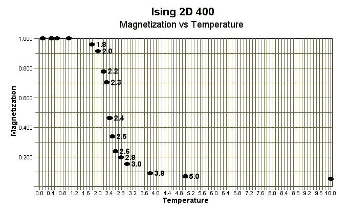
The Magnetization (per spin) vs Temperature plot below was constructed from data obtained with the Ising 2D 400 program. For this relatively small (20×20) lattice, a critical temperature in the range 2.3 to 2.5J was obtained.

This version of the Ising model uses the Metropolis algorithm which was introduced by Nicolas Metropolis and his co-workers in a 1953 paper on simulations of hard-sphere gases.

If there are N sites on the lattice, then the system can be in 2^N states, and the energy of any particular state is given by the Ising Hamiltonian:

where J is an interaction energy between nearest neighbor spins, and B is an external magnetic field. Most of the interesting questions concerning the Ising model can be answered by performing simulations in zero magnetic field B=0, and generalization to the case B not equal to 0 is not hard. Almost all past studies of the Ising model, including Onsager’s exact solution in two dimensions, have looked only at the zero-field case. That is the case considered with Ising 2D 400.

Ising 2D 400 uses an array of 400 variables which take the values 0 or 1, corresponding to ± 1. Periodic boundary conditions have been applied. That is, the spins on one edge of the lattice are neighbors of the corresponding spins on the other edge. This ensures that all spins have the same number of neighbors and local geometry, and that there are no special edge spins which have different properties from the others. All the spins are equivalent and the system is completely translationally invariant.

There are two initial states – the zero-temperature state and the infinite-temperature state. At T=0, the Ising model will be in its ground state. When the interaction energy J is greater than zero and the external field B is zero, there are actually two ground states. These are the states in which the spins are all up or all down. In these states each pair of spins in the first term of the equation above contributes the lowest possible energy –J to the Hamiltonian. In any other state there will be pairs of spins which contribute +J to the Hamiltonian,
and its overall value will be higher. When T=infinity, the thermal energy kT available to flip the spins is infinitely larger than the energy due to the spin-spin interaction J, so the spins are oriented randomly up or down in an uncorrelated fashion.

Since simulations are often performed consecutively at a range of different values of T, it is advantageous to choose as the initial state of the system the final state of the system for a simulation at a nearby temperature.

The first step in the simulation is to generate a new state v that should differ from the present one u by the flip of one spin (an algorithm that does this is said to have single-spin-flip dynamics), and every such state should be exactly as likely as every other to be generated. This is accomplished by picking, at random, a single spin p from the lattice to be flipped. The difference in energy between the new state and the old is then calculated. The only terms in the first term of the Hamiltonian that change are those that involve the flipped spin. The others remain unchanged and so cancel out when the difference E_v – E_u is taken. The change in energy between the two states is thus

In the second line, the sum is over only those spins i of the nearest neighbors of the flipped spin p and all of the spins do not themselves flip, so that s ^v_i = s ^u_i. If s ^u_p = +1, then after spin p has been flipped s ^v_p = -1, so that s ^v_p – s ^u_p  = -2. If s ^u_p = -1, then s ^v_p – s ^u _p  = +2. Thus s ^v_p – s ^u_p  = -2 s ^v_p , and

This involves summing over four terms in the case of a square lattice, where the nearest neighbors are the squares above, below, left and right. If a new state is selected which has an energy lower than or equal to the present one, then the transition to that state should always be accepted. If it has a higher energy then it may be accepted according to the probability

Most of the information here, and that used to construct Ising 2D 400, is from Newman.

References
Newman, M. E. J. and G. T. Barkema Monte Carlo Methods in Statistical Physics
(Clarendon Press, Oxford, 1999) [ ISBN:0-19-851797-1 (Pbk) ].

Yeomans, J. M. Statistical Mechanics of Phase Transitions
(Clarendon Press, Oxford, 1992) [ ISBN:0-19-851730-0 (Pbk) ].

Stanley, H. Eugene Introduction to Phase Transitions and Critical
Phenomena
(Oxford University Press, Oxford, 1987) [ ISBN:0-19-505316-8 (Pbk) ].

Metropolis, N., Rosenbluth, A. W., Rosenbluth, M. N., Teller, A.
H. and Teller, E. 1953 J. Chem. Phys. 21, 1087.

Onsager, L. 1944 Phys. Rev. 65, 117.

Ising 2D 400 Information

Download or save the software by clicking here or on “Ising 2D 400” or the icon on the front page.

Information on how to use the software is here.

The Ising model is a model of a magnet. The essential premise behind it is that the magnetism of a bulk material is made up of the combined magnetic dipole moments of many atomic spins within the material. The model postulates a lattice (can be any geometry) with a magnetic dipole or spin on each site. Ising 2D 400 is so-called because it is a 20×20 (400 sites) two-dimensional Ising model.

In the Ising model the spins assume the simplest form possible (not very realistic) of scalar variables which can take only two values, ± 1, representing up-pointing or down-pointing dipoles of unit magnitude.

Although the Ising model can give answers for the critical properties of a system, the accuracy of the answers depends on the size of the system, with the answers improving steadily as the system size grows. For a system of N spins there are 2^N terms, of which only 2^N-1 need to be calculated.

The critical temperature at which the length-scale of the fluctuations in the magnetization, also called the correlation length, diverges is a non-analytic point at about kT = 2.3J on an infinite lattice as calculated by Onsager.

The Magnetization (per spin) vs Temperature plot below was constructed from data obtained with the Ising 2D 400 program. For this relatively small (20×20) lattice, a critical temperature in the range 2.3 to 2.5J was obtained.

If there are N sites on the lattice, then the system can be in 2^N states, and the energy of any particular state is given by the Ising Hamiltonian:

where J is an interaction energy between nearest neighbor spins, and B is an external magnetic field. Most of the interesting questions concerning the Ising model can be answered by performing simulations in zero magnetic field B=0, and generalization to the case B not equal to 0 is not hard. Almost all past studies of the Ising model, including Onsager’s exact solution in two dimensions, have looked only at the zero-field case. That is the case considered with Ising 2D 400.

Ising 2D 400 uses an array of 400 variables which take the values 0 or 1, corresponding to ± 1. Periodic boundary conditions have been applied. That is, the spins on one edge of the lattice are neighbors of the corresponding spins on the other edge. This ensures that all spins have the same number of neighbors and local geometry, and that there are no special edge spins which have different properties from the others. All the spins are equivalent and the system is completely translationally invariant.

There are two initial states – the zero-temperature state and the infinite-temperature state. At T=0, the Ising model will be in its ground state. When the interaction energy J is greater than zero and the external field B is zero, there are actually two ground states. These are the states in which the spins are all up or all down. In these states each pair of spins in the first term of the equation above contributes the lowest possible energy –J to the Hamiltonian. In any other state there will be pairs of spins which contribute +J to the Hamiltonian,
and its overall value will be higher. When T=infinity, the thermal energy kT available to flip the spins is infinitely larger than the energy due to the spin-spin interaction J, so the spins are oriented randomly up or down in an uncorrelated fashion.

Since simulations are often performed consecutively at a range of different values of T, it is advantageous to choose as the initial state of the system the final state of the system for a simulation at a nearby temperature.

The first step in the simulation is to generate a new state v that should differ from the present one u by the flip of one spin (an algorithm that does this is said to have single-spin-flip dynamics), and every such state should be exactly as likely as every other to be generated. This is accomplished by picking, at random, a single spin p from the lattice to be flipped. The difference in energy between the new state and the old is then calculated. The only terms in the first term of the Hamiltonian that change are those that involve the flipped spin. The others remain unchanged and so cancel out when the difference E_v – E_u is taken. The change in energy between the two states is thus

In the second line, the sum is over only those spins i of the nearest neighbors of the flipped spin p and all of the spins do not themselves flip, so that s ^v_i = s ^u_i. If s ^u_p = +1, then after spin p has been flipped s ^v_p = -1, so that s ^v_p – s ^u_p  = -2. If s ^u_p = -1, then s ^v_p – s ^u _p  = +2. Thus s ^v_p – s ^u_p  = -2 s ^v_p , and

This involves summing over four terms in the case of a square lattice, where the nearest neighbors are the squares above, below, left and right. If a new state is selected which has an energy lower than or equal to the present one, then the transition to that state should always be accepted. If it has a higher energy then it may be accepted according to the probability

Most of the information here, and that used to construct Ising 2D 400, is from Newman.

References
Newman, M. E. J. and G. T. Barkema Monte Carlo Methods in Statistical Physics
(Clarendon Press, Oxford, 1999) [ ISBN:0-19-851797-1 (Pbk) ].

Yeomans, J. M. Statistical Mechanics of Phase Transitions
(Clarendon Press, Oxford, 1992) [ ISBN:0-19-851730-0 (Pbk) ].

Stanley, H. Eugene Introduction to Phase Transitions and Critical Phenomena
(Oxford University Press, Oxford, 1987) [ ISBN:0-19-505316-8 (Pbk) ].

Metropolis, N., Rosenbluth, A. W., Rosenbluth, M. N., Teller, A. H. and Teller, E. 1953 J. Chem. Phys. 21, 1087.

Onsager, L. 1944 Phys. Rev. 65, 117.